Normalizing Flows and Autoregressive Flows
This is a note that I took when I read the MAF paper, NAF paper, Normalizing Flows Tutorials by Eric Jang and its variations by Adam Kosiorek
Machine learning is all about probability. To train a model, we typically tune its parameters to maximize the probability of the training dataset under the model. To do so, we have to assume some probability distribution as the output of our model. The most common one, Gaussian distribution, can be problematic, as the true probability density function (\(pdf\)) of real data is often far from Gaussian. If we use the Gaussian as likelihood for image-generation models, we end up with blurry reconstructions, as proved in Variational Autoencoders (VAEs). We can circumvent this issue by adversarial training, which is an example of likelihood-free inference, but this approach has its own issues.
It is fact that Gaussians are also used, and often prove too simple. Fortunately, we can often take a simple probability distribution, take a sample from it and then transform the sample. This is equivalent to change of variables in probability distributions and, if the transformation meets some mild conditions, can result in a very complex \(pdf\) of the transformed variable. Danilo Rezende formalized this in his paper on Normalizing Flows (NF). NFs are usually used to parametrize the approximate posterior \(q\) in VAEs but can also be applied for the likelihood function.
Change of Variables
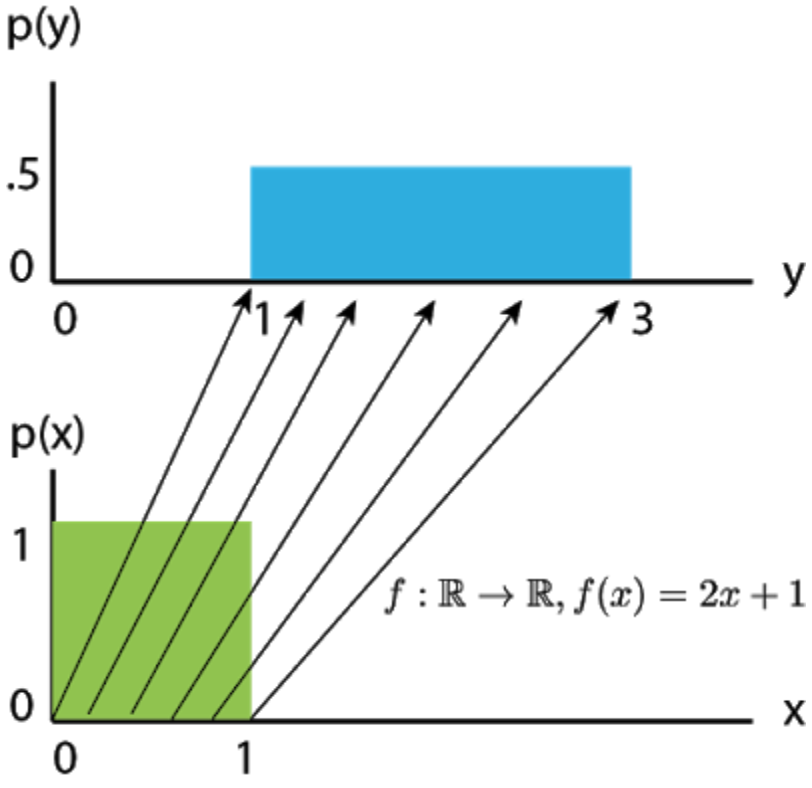
Let’s build up some intuition by examining linear transformations of \(1\)D random variables. Suppose \(X\) is Uniform\((0,1)\). Let random variable \(Y=f(X)=2X+1\) be a simple affine transformation of the underlying “source distribution” \(X\). What this means is that a sample \(x^i\) from \(X\) can be converted into a sample \(y^i\) from \(Y\) by simply applying the function \(f\) to it.

Becasue of the linear transformation, the spanning of \(X\) transforms from \([0, 1] \text{ to } [1, 3]\). Since the probability mass must integrate to \(1\) for both distributions, we have density \(p(x) = 1 \text{ and } p(y) = 0.5\)
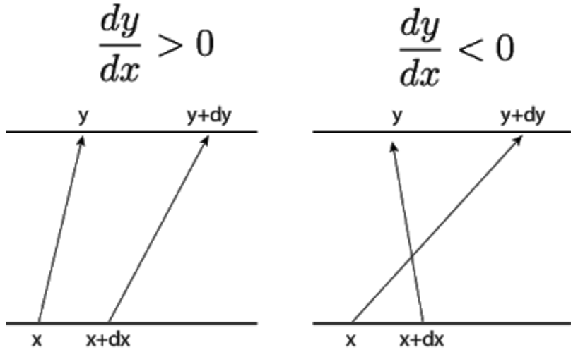
Let’s zoom in on a particular \(x\) and an infinitesimally nearby point \(x+dx\), then applying \(f\) to them takes us to the pair \((y,y+dy)\).

That being said, to preserve the total probability (\(=1\)), the change of \(p(x)\) along \(dx\) must be equivalent to the change of \(p(y)\) along \(dy\) :
\[p(x)\left|dx\right| = p(y)\left|dy\right| \tag{1}\]Then, we have the density after transformation \(p(y) = p(x)\left|\frac{dx}{dy}\right|\)
To make it numerical stabler, we often take \(log\).
\[\text{log} \ p(y) = \text{log} \ p(x) + \text{log}\left|\frac{dx}{dy}\right| \tag{2}\]
Now, let’s look at multivariate case, specifically with 2 variabels.

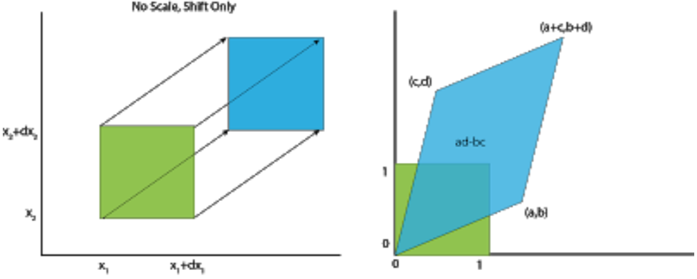
We have a square from four initial vertices \((0,0), (0,1), (1,0), (1,1)\). After appling the matrix transformation \(\begin{bmatrix}a & b\\c & d\end{bmatrix}\), they are taken into a parallelogram and each vertice is sent to \((0,0), (c,d), (a,b), (a+c,b+d)\) respectively.
Thus, the area \(dA = 1\) changes to \(dA = ad-bc\). It’s important to notice that \(ad-bc\) is nothing but the determinant of the linear transformation.
Mathematically,
\[\begin{align} p(y) &= p(f^{-1}(y)) \cdot \left|\text{det} J(f^{-1}(y))\right| \\ &= p(x) \cdot \left|\text{det} J(f^{-1}(y))\right| \tag{3} \\ \end{align}\]Notice: As far, we just explore linear transformation, which is the simplest case. Non-linear transformation is essentially the same but just need to meet one condition: bijection (linear transformation is for sure invertible).
In Danilo’s paper, let \(\mathbf{z} \in \mathbb{R}\) be a random variable and \(f :\mathbb{R}^d \mapsto \mathbb{R}^d\) an invertible smooth mapping. We can use \(f\) to transform \(\mathbf{z}∼q(\mathbf{z})\). The resulting random variable \(\mathbf{y}=f(\mathbf{z})\) has the following probability distribution:
\[\begin{align} q_y(\mathbf{y}) &= q(\mathbf{z}) \left| \text{det} \frac{\partial{f^{-1}}}{\partial{\mathbf{z}}} \right|\\ &= q(\mathbf{z}) \left| \text{det} \frac{\partial{f}}{\partial{\mathbf{z}}} \right|^{-1} \tag{4} \\ \end{align}\]We can apply a series of invertible mappings \(f_k, k \in 1, ... ,K, \text{with } K \in \mathbb{N_+}\) and obtain a normalizing flow.
\[\mathbf{z} = f_K \circ \cdots \circ f_1(\mathbf{z}_0), \qquad \mathbf{z}_0 \sim q_0(\mathbf{z}_0) \tag{5}\] \[\mathbf{z} \sim q_K(\mathbf{z}_K) = q_0(\mathbf{z}_0) \prod_{k=1}^{K} \left| \text{det} \frac{\partial{f_k}}{\partial{\mathbf{z_k}}} \right|^{-1}\tag{6}\]This series of transformations can transform a simple probability distribution (e.g. Gaussian) into a complicated multi-modal one. To be of practical use, however, we can consider only transformations whose determinants of Jacobians are easy to compute. The original paper considered two simple family of transformations, named planar and radial flows.
- Planar Flow
where \(\lambda = \{\mathbf{u}, \mathbf{w} \in \mathbb{R}^d, b \in \mathbb{R}\}\) are free parameters, and h is a smooth element-wise non-linearity. We can then compute the logdet-Jacobian term in \(O(D)\) time using the matrix determinant lemma:
\[\psi(\mathbf{z}) = h^{\prime}(\mathbf{w}^{\intercal}\mathbf{z} + b)\mathbf{w}\] \[\left| \text{det} \frac{\partial{f}}{\partial{\mathbf{z}}} \right| = \left| \text{det}({\mathbf{I} + \mathbf{u} \psi(\mathbf{z}))^{\intercal}} \right|= \left| 1 + \mathbf{u}^{\intercal} \psi(\mathbf{z}) \right| \tag{8}\]We conclude that the log density \(q_K(\mathbf{z})\) obtained by transforming an arbitraty initial density \(q_0(\mathbf{z})\) through the sequence of maps \(f_k\) is implicitly given by:
\[\text{ln } q_K(\mathbf{z_K}) = \text{ln } q_0(\mathbf{z}) - \sum_{k=1}^K \text{ln } \left| 1 + \mathbf{u_k}^{\intercal} \psi_k(\mathbf{z_k}) \right| \tag{9}\]The flow defined by \((9)\) modifies the initial density \(q_0\) by applying a series of contractions and expansions in the direction perpendicular to the hyperplane \(\mathbf{w}^{\intercal}\mathbf{z} + b = 0\), hence we refer to these maps as planar flows.
- Radial Flow
As an alternative, we can consider a family of transformation that modify an initial density \(q_0\) around a reference point \(\mathbf{z}_0\)
\[f(\mathbf{z}) = \mathbf{z} + \beta h(\alpha, r)(\mathbf{z}-\mathbf{z_0})\tag{10}\]where \(r = |\mathbf{z} - \mathbf{z_0}|, h(\alpha, r) = \frac{1}{\alpha+r} \text{ and parameters are } \lambda = \{ \mathbf{z_0} \in \mathbb{R}^d, \alpha \in \mathbb{R}, \beta \in \mathbb{R} \}\)
This family allows for a linear-time computation of the determinant.
\[\left| \text{det} \frac{\partial{f}}{\partial{\mathbf{z}}} \right| = \left[ 1 + \beta h(\alpha, r) \right]^{d-1} \left[ 1 + \beta h(\alpha, r) + h^{\prime}(\alpha, r)r \right] \tag{11}\]
Discussion
Here is the result of two families on Gaussian and Uniform distribution.

These simple flows are useful only for low dimensional spaces, since each transformation affects only a small volume in the original space. As the volume of the space grows exponentially with the number of dimensions \(d\), we need a lot of layers in a high-dimensional space.
Another way to understand the need for many layers is to look at the form of the mappings. Each mapping behaves as a hidden layer of a neural network with one hidden unit and a skip connection. Since a single hidden unit is not very expressive, we need a lot of transformations. Recently introduced Sylvester Normalizing Flows overcome the single-hidden-unit issue of these simple flows.
Autoregressive Flows
Enhancing expressivity of normalizing flows is not easy, since we are constrained by functions, whose Jacobians are easy to compute. It turns out, though, that we can combine it with autoregressive model. We introduce dependencies between different dimensions of the latent variable, and still end up with a tractable Jacobian. Namely, if after a transformation, the dimension \(i\) of the resulting variable depends only on demension \(1 : i\) of the input variable, then the Jacobian of this transformation is triangular. As we know, a determinant of a triangular matrix is equal to the product of the terms on the diagonal. More formally, let \(J \in \mathbb{R}^{d\text{x}d}\) be the Jacobian of the mapping \(f\), then
\[y_i = f(\mathbf{z}_{1:i}) \qquad J = \frac{\partial{\mathbf{y}}}{\partial{\mathbf{z}}} \tag{12}\] \[\text{det} J = \prod_{i=1}^d J_{ii} \tag{13}\]Here are four flows that use the above concept, albeit in different ways, and arrive at mappings with very different properties.
- Real Non-Volume Preserving Flows (R-NVP)
R-NVPs are arguably the least expressive but the most generally applicable of the three. Let \(1 < k < d\), \(\odot\) element-wise multiplication and \(\mu\) and \(\sigma\) two mappings (through neural networks) \(\mathbb{R}^k \mapsto \mathbb{R}^{d-k}\) (Note that \(\sigma\) is not the sigmoid function). What’s called Coupling layer that transforms a density to another density is defined as:
\[\mathbf{y}_{1:k} = \mathbf{z}_{1:k} \tag{14}\] \[\mathbf{y}_{k+1:d} = \mathbf{z}_{k+1:d} \odot \text{exp }\sigma(\mathbf{z}_{1:k}) + \mu(\mathbf{z}_{1:k}) \tag{15}\]It is an autoregressive transformation, although not as general as equation \((13)\) allows. It copies the first \(k\) dimensions, while shifting and scaling all the remaining ones. The first part of the Jacobian(up to dimension \(k\)) is just an identity matrix, while the second part is lower-triangular with \(\sigma(\mathbf{z}_{1:k})\) on the diagonal. Hence, the determinant of the Jacobian is
\[\frac{\partial{\mathbf{y}}}{\partial{\mathbf{z}}} = \prod_{i=1}^{d-k}\sigma_i(\mathbf{z}_{1:k}) \tag{16}\]R-NVPs are particularly attractive because both sampling and inference are equally efficient. This allows to use R-NVPs as a parametrization of an approximate posterior \(q\) in VAEs, but also as the output likelihood (in VAEs or general regression models). To see this, first note that we can compute all elements of \(\mu\) and \(\sigma\) in parallel, since all inputs (\(\mathbf{z}\)) are available. We can therefore compute \(\mathbf{y}\) in a single forward pass. Next, note that the inverse transformation has the following form, with all divisions done element-wise,
\[\mathbf{z}_{1:k} = \mathbf{y}_{1:k} \tag{17}\] \[\mathbf{z}_{k+1:d} = \frac{\mathbf{y}_{k+1:d}-\mu(\mathbf{y}_{1:k})}{\sigma({\mathbf{y}_{1:k}})}\]Note that \(\mu\) and \(\sigma\) are usually implemented as Neural networks, which are generally not invertible. Thanks to equation \((17)\), however, they do not have to be invertible for the whole R-NVP transformation to be invertible. Notice that with a single coupling layer, some components are unchanged in forward transformation. In original paper, this problem is overcome by stacking multiple coupling layers and permute the ordering of copied dimensions. The Jacobian determinant remains tractable.
Autoregressive models as normalizing flows
We can be even more expressive than R-NVPs. Consider an autoregressive model whose conditionals are parameterize as single Gaussian. That is, the \(i^{th}\) conditional is given by
\[p(x_i|\mathbf{x}_{1:i-1}) = \mathcal{N} (x_i|\mu_i, (\text{exp } \sigma_i)^2) \tag{18}\]where \(\mu_i\) and \(\sigma_i\) are unconstraied scalar functions(through neural nets) that compute the mean and log standard deviation of the \(i^{th}\) conditional given all previous variables. Thus,we can generate data from the above model using the following recursion:
\[x_i = u_i \text{ exp }{\sigma_i} + \mu_i \tag{19}\]where \(u_i \sim \mathcal{N}(0,1)\) and \(\mathbf{u} = (u_1, u_2, ..., u_K)\) is the vecotr of random numbes the model uses internally to generate data.
\((19)\) provides an alternative characterization of the autoregressive model as a transformation \(f\) from the space of random numbers \(\mathbf{u}\) to the space of data \(\mathbf{x}\). That is, we can express the model as \(\mathbf{x} = f(\mathbf{u})\). Given a datapoint \(\mathbf{x}\), the random numbers \(\mathbf{u}\) that were used to generate it are obtained by:
\[u_i = (x_i-\mu_i) \text{exp} (-\sigma_i) \tag{20}\]Due to the autoregressive structure, the Jacobian of \(f^{-1}\) is triangular by design, hence its absolute determinant can be easily obtained as follows:
\[\left| \text{det} \left( \frac{\partial{f^{-1}}}{\partial{\mathbf{x}}} \right) \right| = \text{exp} \left( -\sum_i \sigma_i \right) \tag{21}\]- Masked Autoregressive Flow (MAF)
MAF directly uses equations \((18)\) and \((19)\) to transform as random variable. It is named Masked because it used Masked Autoencoder for distribution Estimation (MADE) as a building block. Specifically, we choose to implement the set of functions \({\mu, \sigma}\) with masking. The benefit of using maskng is that it enables transforming from data \(\mathbf{x}\) to random numbers \(\mathbf{u}\) and thus calculating \(p(\mathbf{x})\) in one forward pass through the flow, thus eliminating the need for sequential recursion in \((20)\). In practice, we adds flexibility to this model by stacking multiple instances of the model into a deeper flow.
- Inverse Autoregressive Flow (IAF)
Like MAF, IAF is a normalizing flow which uses MADE as its component layer. Each layer of IAF is defined by the following resursion:
\[x_i = u_i \text{ exp } \sigma_i + \mu_i \tag{22}\]Similar to MAF, functions \({\mu_i, \sigma_i}\) are computed using a MADE with Gaussian conditionals. The difference is architectural: in MAF \(\mu_i\) and \(\sigma_i\) are directly computed from previous data variables \(\mathbf{x}_{1:i-1}\), whereas in IAF \(\mu_i\) and \(\sigma_i\) are directly computed from precious random numbers \(\mathbf{u}_{1:i-1}\)
where \(\mu_i\) and \(\sigma_i\) are unconstraied scalar functions(through neural nets) that compute the mean and log standard deviation of the \(i^{th}\) conditional given all previous variables.
MAF v.s IAF
It’s important to know the trade-off of MAF and IAF as they present different consequences. MAF is capable of calculating the density \(p(\mathbf{x})\) of any datapoint \(\mathbf{x}\) in one pass through the model, however samping from it requires performing D sequential passes (D is the dimensionality of \(\mathbf{x}\)). This can be seen from \((20)\) and \((21)\) that they can be immediately used in exact density estimation:
\[p(x) = p(u) \left| \text{det} \left( \frac{\partial{f^{-1}}}{\partial{\mathbf{x}}} \right) \right| \tag{23}\]where \(p(u)\) is the base/unstructured distribution that is easy to compute. In this post, we use standard normal.
In contrast, for IAF calculating the density \(p(\mathbf{x})\) of externally provided datapint \(\mathbf{x}\) requires D passes to find the random number \(\mathbf{u}\) associated with \(\mathbf{x}\) because \(u_i\) depends on the computation of previous \(u_{1:i-1}\). However, IAF can generate samples and calculate their density with one pass since all the \(x_i\) can be computed in a sinle pass of \(D\) threads in parallel. Hence, the design choice depends on the intended usage. IAF is suitable as a recognition model for stochastic variational inference, where it only ever needs to calculate the density of its own samples. In contrast, MAF is more suitable for density estimation, because each example requires only one pass through the model.
Neural Autoregressive Flows (NAF)
This is a relatively state-of-the-art work by Huang, et al., which substantially improve the above-mentioned autoregressive flows in terms of expressiveness.
Let’s recall what we got so far from IAF and MAF. Our initial motivation is that autoregressive model can be combined with normalizing flows to produce good results in density estimation and that different ways to combine these two, as shown in IAF and MAF, give us different results, depending the usage case. However, both IAF and MAF limit themsleves with affine transformation throughout normalizing flows for computational simplicity. For instance, \(x_i = u_i \text{ exp }{\sigma_i} + \mu_i\).
One problem of this restriction is that because of this restriction, we are limiting ourselves in a small family of functions, and thus a small famil of densities. However, we observed that for computational simplicity, we just need to satisfy two requirements:
- transforming functions are invertible w.r.t \(x_i\)
- \(\frac{dy_i}{dx_i}\) is cheap to compute
This raised the possibility to using a more poweful transformation in order to increase the expressivity of the flow.
We define an autoregressive conditioner c, and an invertible transformer \(\tau\), and then the function that transform \(x_i\) to \(y_i\) is defined as:
\[y_i = f(x_{1:i}) = \tau(c(x_{1:i-1}), x_i) \tag{24}\]In NAF, we replace the affine transformer with a neural network, and yields a more rich family of distributions with only a minor increae in computation and memory requirements:
\[\tau(c(x_{1:i-1}), x_i) = \text{DNN}(x_i; \phi=c(x_{1:i-1})) \tag{25}\]where in deep neural network, \(x_i\) is input, \(y_i\) is output and its weights and biases are given by the output of \(c(x_{1:i-1})\)
Now the question is, how to make sure that the two requirements for computational simplicity are satisfied?
In original paper, the author makes the network to be monotonic by forcing strictly positive weights and strictly monotonic activation functions for \(\tau_i\). Strictly monotonic NAF will thus be invertible (as per requirement \(1\)). Meanwhile, \(\frac{dy_i}{dx_i}\) and gradients w.r.t to parameters can be computed efficiently via backpropagation (as per requirement 2).
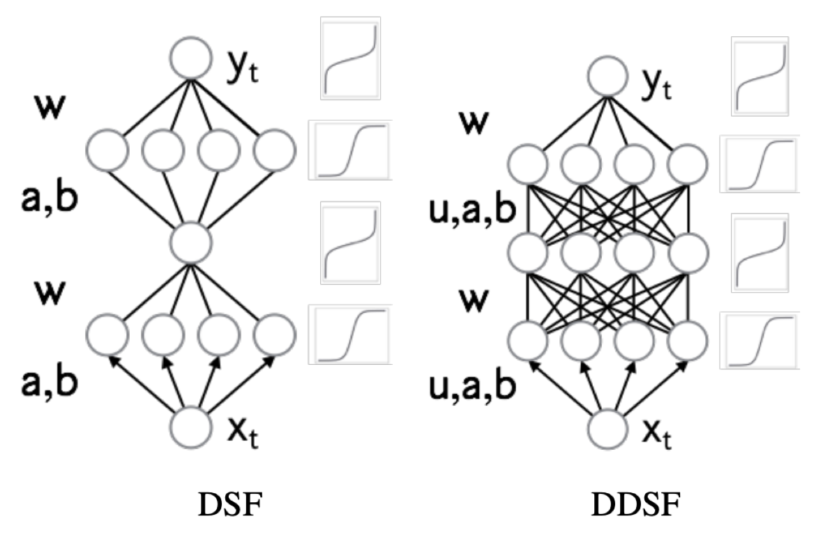
Two neural architectures for \(\tau_i\) is proposed performing well: deep sigmoidal flows (DSF) and deep dense sigmoidal flows (DDSF)

Summary
In this article, I attempt to understand a) what is normalizing flows, b) what is the mathematical background of this normallizing flows, c) R-NVP that utilizes deep normalizing flows, d) two generalization of R-NVP–MAF and IAF–that use autoregressive models as normalizing flows, called autoregressive flows.
Moreover, I demonstrate the pros and cons of R-NVP, MAF, and IAF, depending on the intention of usage:
-
MAF can calculate the density \(p(\mathbf{x})\) in a single pass so it’s useful for explicit density estimation. However, it takes D passes to generate the data, thus not suitable for variational inference.
-
IAF, on the other hand, can generate data in single pass but is slow in computing density \(p(\mathbf{x})\)
-
R-NVP, is a special case of MAF but the benefits of it is that it can both generate data and estimate densities with one forward pass only.