CNN Architectures
In this post, I will introduce some popular CNN architectures
LeNet-5
Before CNN was invented, character recognition had been done mostly by using feature engineering by hand, followed by a machine learning model to learn to classify hand engineered features. In \(1998\), Yann Lecun first proposed a neural network architecture for handwritten and machine-printed character recognition–LeNet. LeNet made hand engineering features redundant, because the network learns the best internal representation from raw images automatically.
LeNet-\(5\) is a very simple network from the point of current standards. It only has \(7\) layers, amomng which are \(3\) convolutional layers(C\(1\), C\(3\), C\(5\)), \(2\) pooling layers(S\(2\), S\(4\)), \(1\) fully connected layer(F6) and an output layer.
 LeCun et al., \(1998\)
C\(1\)
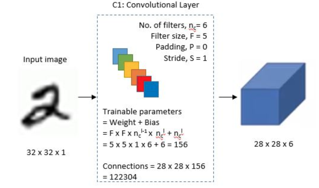
The input for LeNet-\(5\) is a \(32\)x\(32\) grayscale image which is passed through the first convolutional layer(C\(1\)) with \(6\) filters(a.k.a convolutional kernels, or receptive fileds) having size \(5\)x\(5\) and a stride of \(1\). The image is then changed from \(32\)x\(32\)x\(1\) to \(28\)x\(28\)x\(6\)
S\(2\)
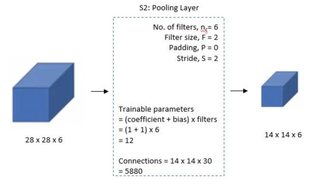
Then the LeNet-\(5\) applies average pooling layer with a filter size \(2\)x\(2\) and a stride of \(2\). The resulting image dimensions will be reduced to \(14\)x\(14\)x\(6\)
C\(3\)
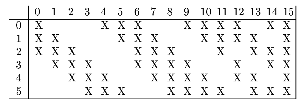
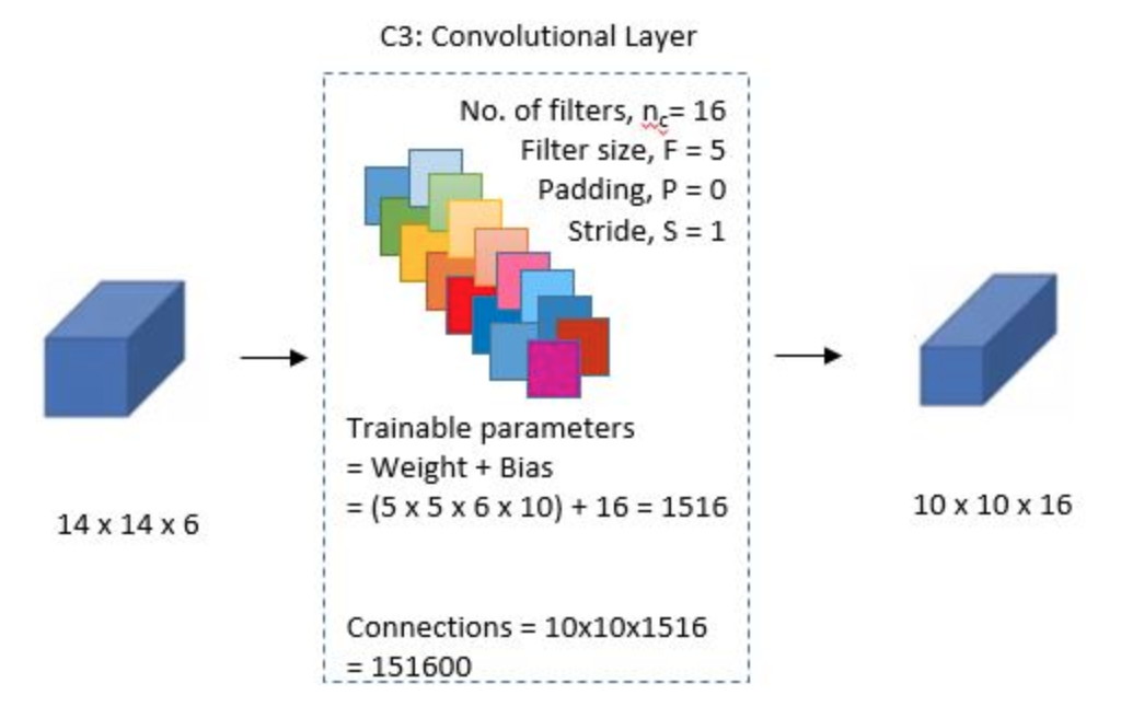
Next, there is a second convolutional layer with \(16\) filters having size \(5\)x\(5\) and a stride of \(1\). In this layer, only \(10\) out of \(16\) filters are connected to \(6\) previous feature maps, as shown below:
 LeCun et al., \(1998\)
The reason for not fully connecting is to break the symmetry in the network and to keep the number of connections within reasonable bounds.
S\(4\)
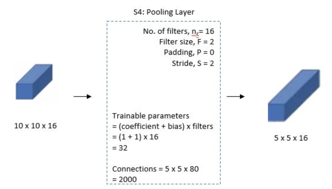
THe fourth layer is again an average pooling layer with filter size \(2\)x\(2\) and a stride of \(2\). This layer is the same as S\(2\) and the output would be \(5\)x\(5\)x\(16\)
C\(5\)
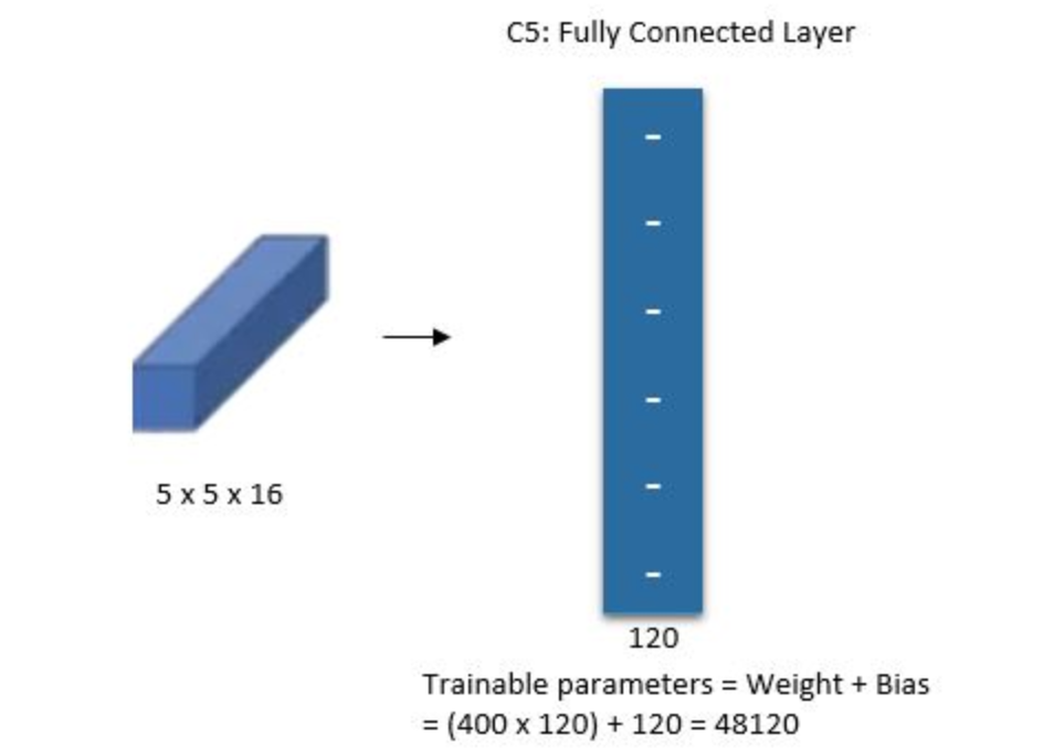
The fifth layer is a fully connected convolutional layer with \(120\) filters each of size \(1\)x\(1\). Each of the \(120\) units in C\(5\) is connected to all the \(400\) node(\(5\)x\(5\)x\(16\)) in the fourth layer S\(4\).
F\(6\)
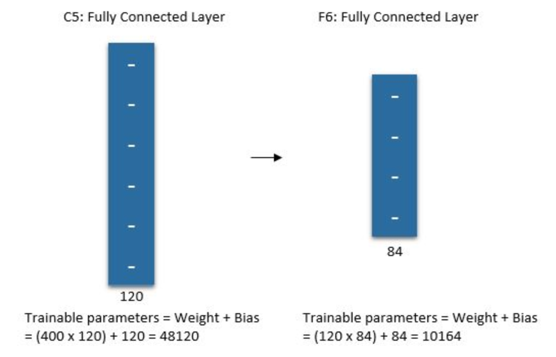
The sixth layer is a fully connected layer with \(84\) units.
Output layer
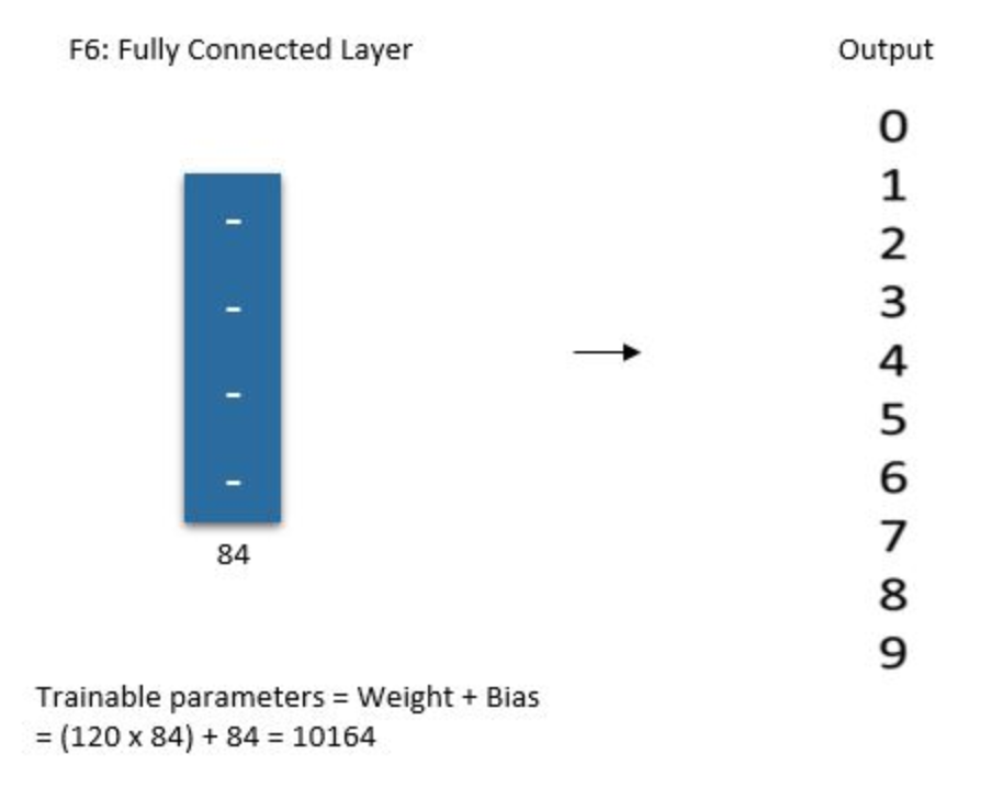
The final layer is a fully connected softmax output layer \(\hat y\) with \(10\) possible values corresponding to the digits from \(0\) to \(9\).
AlexNet
Within more than a decade after LeCun proposed LeNet-\(5\), due to the low expressivity of neural net as well as inefficient computating power, neural nets had been making slow progress. This trough continued for many years until landscape AlexNet won the ILSVRC-\(2012\) with a top-\(5\) error of \(15.3\)% and outperformed the runner up by \(10.8\)% error point.
AlexNet inherented the idea of LeNet-\(5\) but it expanded the neural nets much deeper. Compared to only \(60\)k parameters in LeNet-\(\), AlexNet has \(60\)M parameters, \(650\)k neurons, and \(630\)M connections. AlexNet has \(8\) layers(not including pooling layers), among which are \(5\) convolutional layers and \(3\) fully connected layers. Importantly, AlexNet uses max pooling instead of average pooling and are only applied after the \(1^{st}, 2^{nd}, \text{and} \ 5^{th}\) convolutional layers.
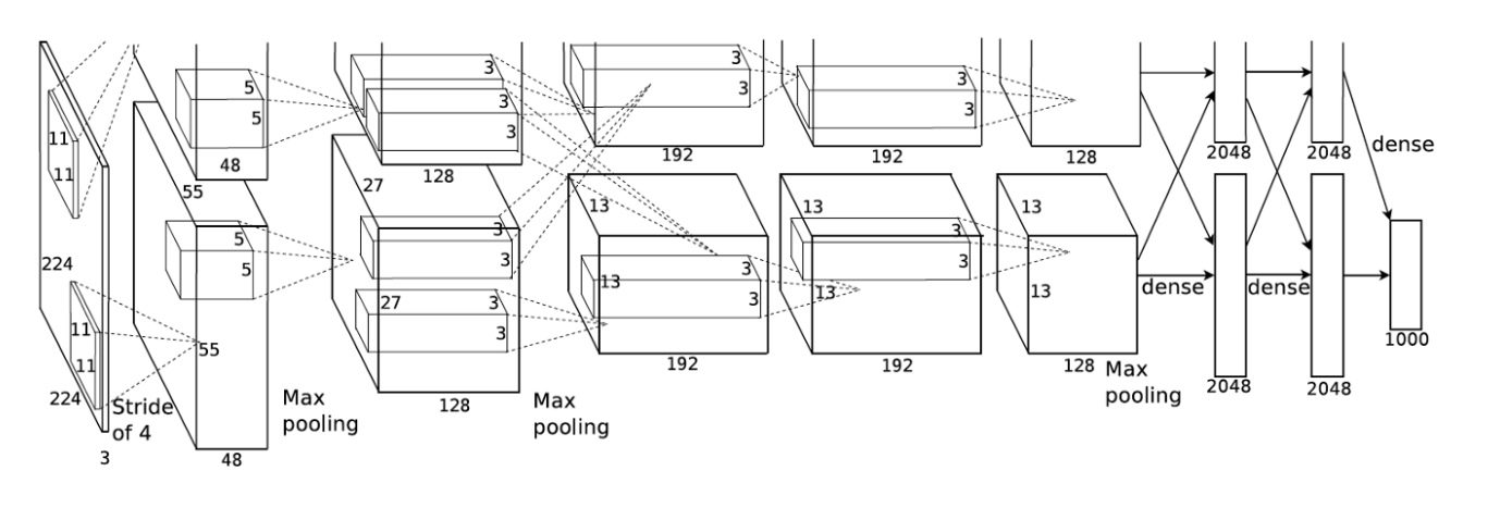 Krizhevsky et al., \(2012\)
Let’s look at this architecture closely.
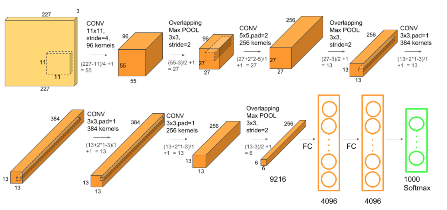
Multiple filters extract interesting features in an image. In a single convolutional layer, there are usually many filters of the same size. For example, the first Conv Layer of AlexNet contains 96 filters of size \(11\)x\(11\)x\(3\). Note the width and height of the filter are usually the same and the depth is the same as the number of channels(here we have \(3\) channels).
The first two Convolutional layers are followed by the Overlapping Max Pooling layers. The third, fourth and fifth convolutional layers are connected directly. The fifth convolutional layer is followed by an Overlapping Max Pooling layer, the output of which goes into a series of two fully connected layers. The second fully connected layer feeds into a softmax classifier with \(1000\) class labels.
ReLU nonlinearity is applied after all the convolution and fully connected layers. The ReLU nonlinearity of the first and second convolution layers are followed by a local normalization step before doing pooling. But researchers later didn’t find normalization very useful. So we will not go in detail over that.
Highlights of AlexNet:
-
Use ReLU as activation function, which has better effect than Sigmoid by preventinbg vanishing gradient
-
Use dropout in fully connected layer to prevent overfitting
-
Use Max pooling instead of average pooling to prevent blur
-
Use multiple GPU to parallelly compute
-
Use data augmentation to prevent overfitting
How to reduce overfitting
AlexNet uses two methods to reduce overfitting.
- Data Augmentation
Showing a Neural Net different variation of the same image helps prevent overfitting. You are forcing it to not memorize! Often it is possible to generate additional data from existing data for free! Here are few tricks used by the AlexNet team.
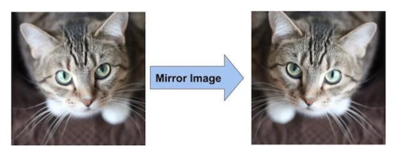
Data Augmentation by Mirroring
If we have an image of a cat in our training set, its mirror image is also a valid image of a cat
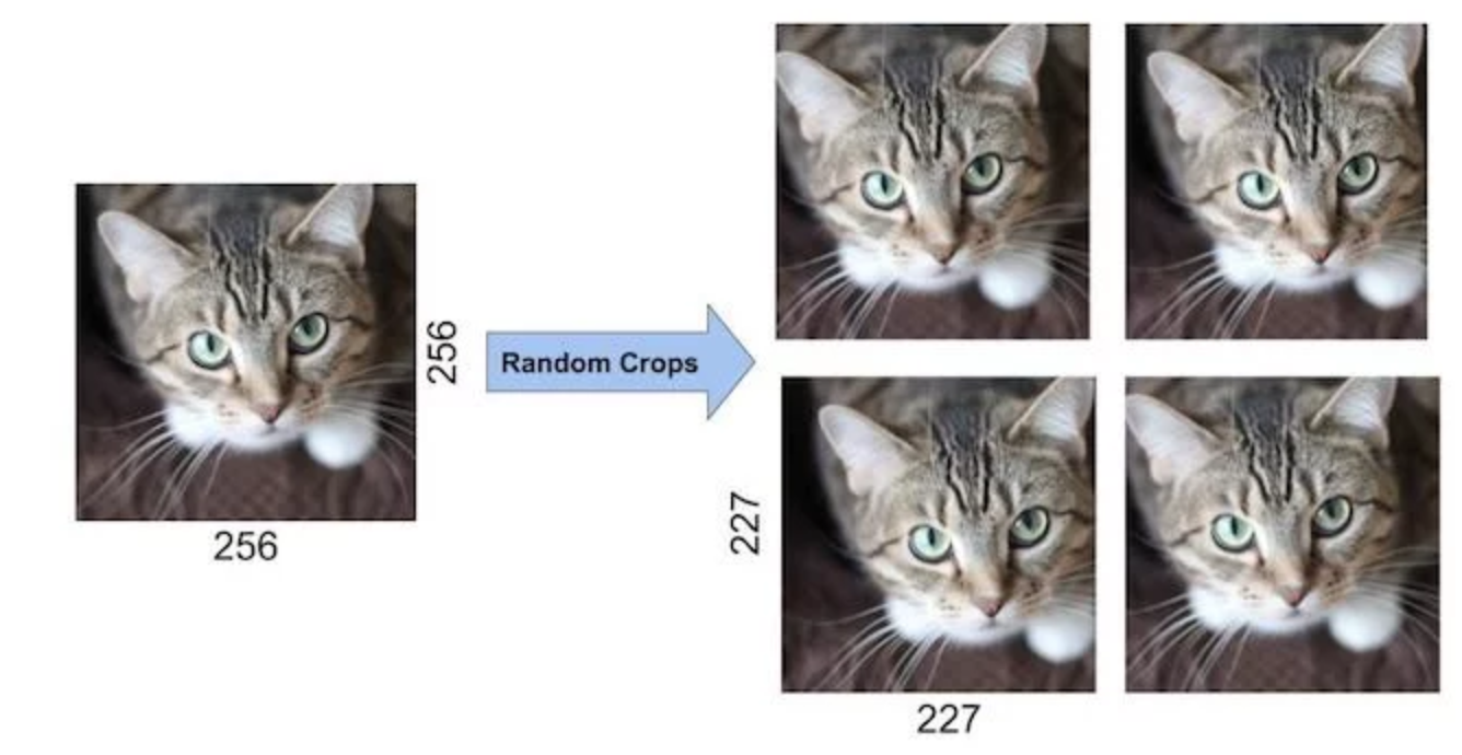
Data Augmentation by Random Crops
In addition, cropping the original image randomly will also lead to additional data that is just a shifted version of the original data.
- Dropout
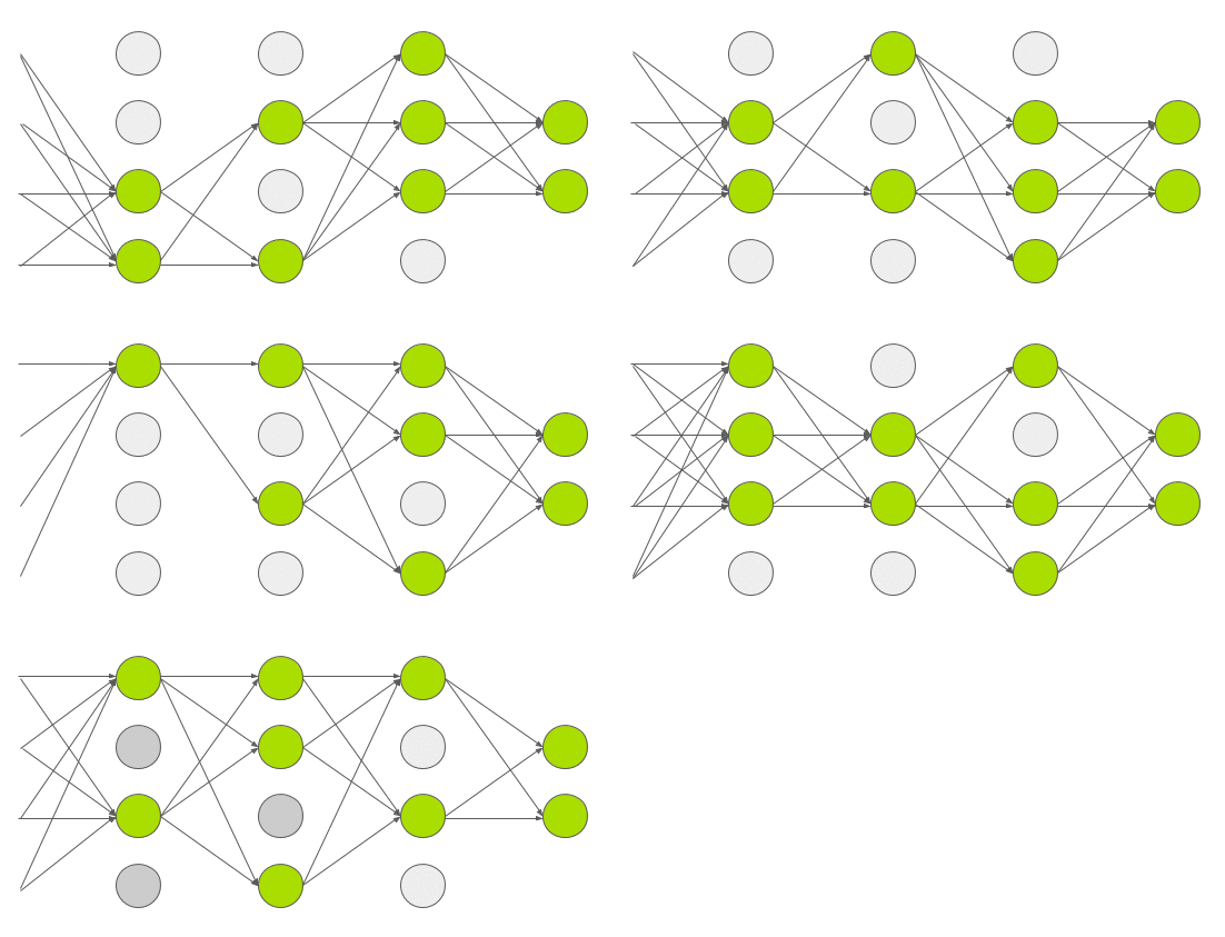
Dropout is a technique introduced by G.E. Hinton in another paper in \(2012\). In dropout, a neuron is dropped from the network with a probability of \(0.5\). When a neuron is dropped, it does not contribute to either forward or backward propagation. So every input goes through a different network architecture, as shown in the animation below. As a result, the learnt weight parameters are more robust and do not get overfitted easily. During testing, there is no dropout and the whole network is used, but output is scaled by a factor of \(0.5\) to account for the missed neurons while training. Dropout increases the number of iterations needed to converge by a factor of \(2\), but without dropout, AlexNet would overfit substantially.
AGGNet
ZFNet won the ILSVRC-\(2013\) but since it was almost the same as AlexNet except for some size and stride change, I wont’t talk about it in thins article. And then in ILSVRC-\(2014\), we have two very close winners: VGGNet achieved error of \(7.3\)% and GoogleNet achieved of \(6.7\)%. Let’s first look at VGGNet and then I will talk about GoogleNet in a bit.
For the big pictute, VGGNet uses smaller filters and deeper networks. Usually, when people are talking VGGNet, they are refering to VGGNet-\(16\) or VGGNet-\(19\), which differ in that VGGNet-\(16\) uses \(16\) layes while VGGNet-\(19\) usese \(19\) layers. Yet they both use \(3\)x\(3\)x\(3\) filters.
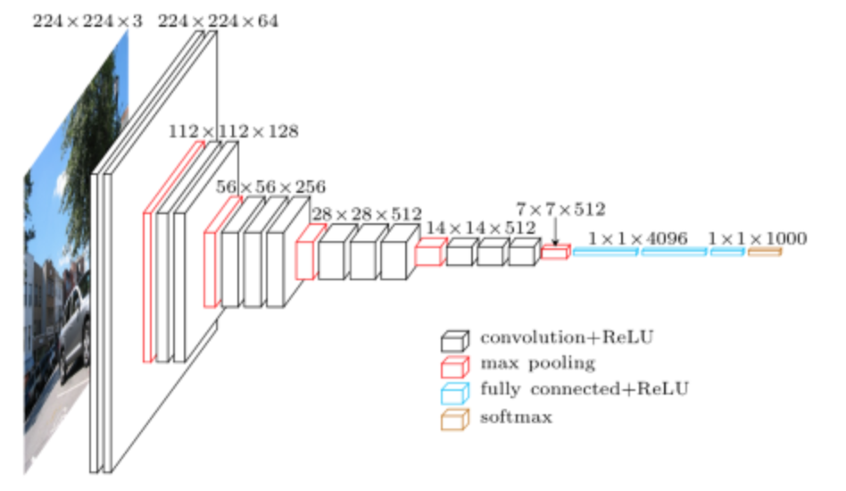
VGGNet uses \(5\) convolutional layers each followed by a max pooling layer, \(3\) fully connected layers, and a Softmax output layer. All activation functions are ReLU.
Highlights of VGGNet:
-
Use smaller \(3\)x\(3\) filters instead of large \(11\)x\(11\) or \(7\)x\(7\)
-
Use Multi-Scale Training
-
Dense Testing
-
No local response normalization(LRN) since it does not improve much
Why do we use smaller layers?
- No need to use large size filters
 By using \(2\) layers of \(3\)×\(3\) filters, it actually have already covered \(5\)×\(5\) area as in the above figure. By using \(3\) layers of \(3\)×\(3\) filters, it actually have already covered \(7\)×\(7\) effective area. Actually, the size of the effective receptive field of a N convolutional layers stack with \(3\)×\(3\) filters is equal to (\(2\)N+\(1\))x(\(2\)N+\(1\)) Thus, large-size filters such as \(11\)×\(11\) in AlexNet and \(7\)×\(7\) in ZFNet indeed are not needed.
- Number of parameters are fewer. Suppose there is only \(1\) filter per layer, \(1\) layer at input, and exclude the bias:
\(1\) layer of \(11\)×\(11\) filter, number of parameters = \(11\)×\(11\)=\(121\)
\(5\) layer of \(3\)×\(3\) filter, number of parameters = \(3\)×\(3\)×\(5\)=\(45\)
Number of parameters is reduced by \(63%\)
\(1\) layer of \(7\)×\(7\) filter, number of parameters = \(7\)×\(7\)=\(49\)
\(3\) layers of \(3\)×\(3\) filters, number of parameters = \(3\)×\(3\)×\(3\)=\(27\)
Number of parameters is reduced by \(45%\)

- More non-linearities
How does multi-scaling work?
As object has different scale within the image, if we only train the network at the same scale, we might miss the detection or have the wrong classification for the objects with other scales. To tackle this, authors propose multi-scale training.
For single-scale training, an image is scaled with smaller-size equal to \(256\) or \(384\). Since the network accepts \(224\)×\(224\) input images only, the scaled image will be cropped to \(224\)×\(224\). The concept is as follows:
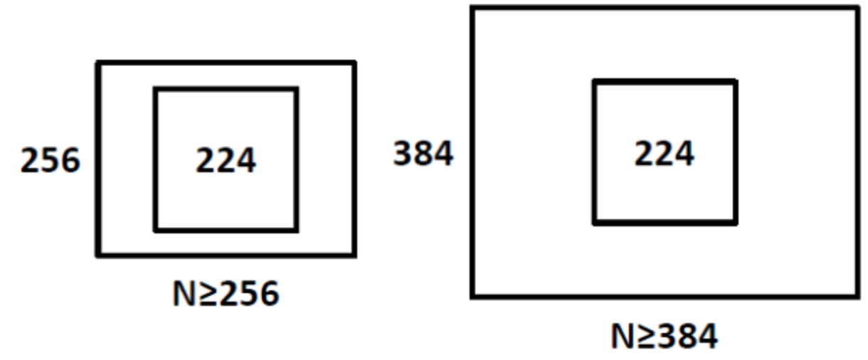
For multi-scale training, an image is scaled with smaller-size equal to a range from \(256\) to \(512\), i.e. S=[\(256\);\(512\)], then cropped to \(224\)×\(224\). Therefore, with a range of S, we are inputting different scaled objects into the network for training.
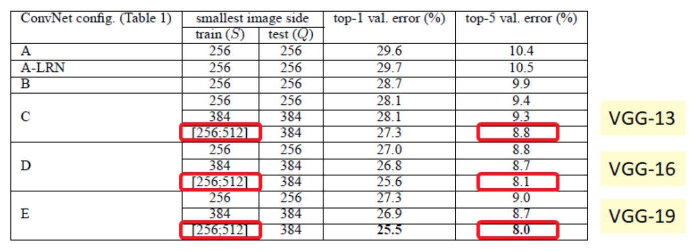
By using multi-scale training, we can imagine that it is more accurate for test image objects with different object sizes.
- VGG-13 reduced the error rate from \(9.3\)% to \(8.8\)%
- VGG-16 educed the error rate from \(8.7\)% to \(8.1\)%
- VGG-19 reduced the error rate from \(8.7\)% to \(8.0\)%
What is Dense Testing?
During testing, VGGNet replace all \(3\) fully connected layers by \(3\) convolutional layers. This is to relax the limit of input image size so that neural nets can accept input of any height and width and this is vital in testing.
If we keep fully connected layers, images should be subject to \(224\)x\(224\)x\(3\) to satisfy fixed size vector.

In VGGNet, the first FC is replaced by \(7\)×\(7\) conv. The second and third FC are replaced by \(1\)×\(1\) conv.

GoogleNet
GoogleNet won ILSVRC-2014 with a slightly better result compared to VGGNet. It is a little bot deeper with \(22\) layers and abandons the fully connected layers.
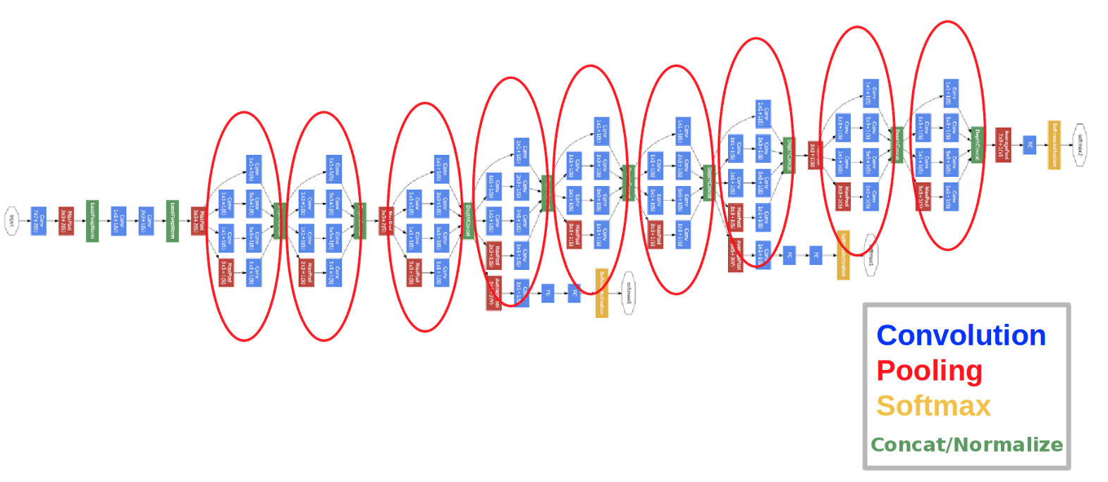
Highlights
-
No FC layers
-
Use efficient “Inception” module
What is Inception module?
Inception module is a local network topology that combines different convolutional layers and a max polling layer in parallel and then concatenate their results depth-wise and then stack many of these modules to form the whole neural net.
Here is a naive way of doing this
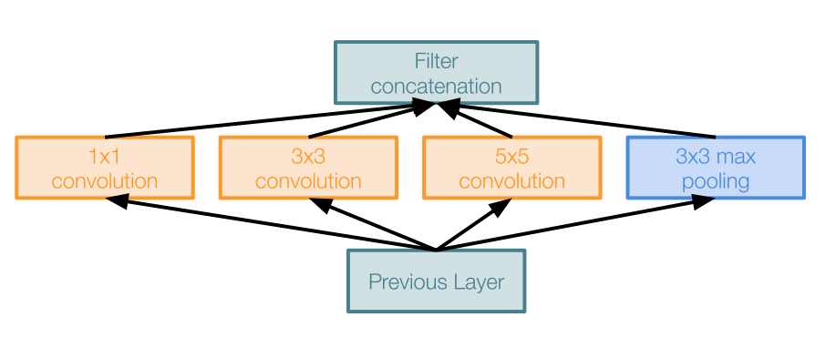
The problem of this naive inception module is huge computaional complexity. For example we have a input of \(28\)x\(28\)x\(256\) (this is not the initial input to the whole net; it is just the local input from previous module).We use zero padding when needed to maintain the same feature map size in order for depth-wise concatenation.

We see that it is very expensive to compute. So we apply a bottleneck layer that use \(1\)x\(1\) convolutions to reduce feature depth.
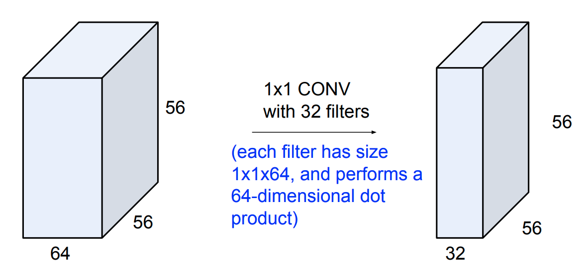
\(\qquad \qquad \qquad \qquad \qquad \qquad \quad \downarrow\)

\(\qquad \qquad \qquad \qquad \qquad \qquad \quad \downarrow\)
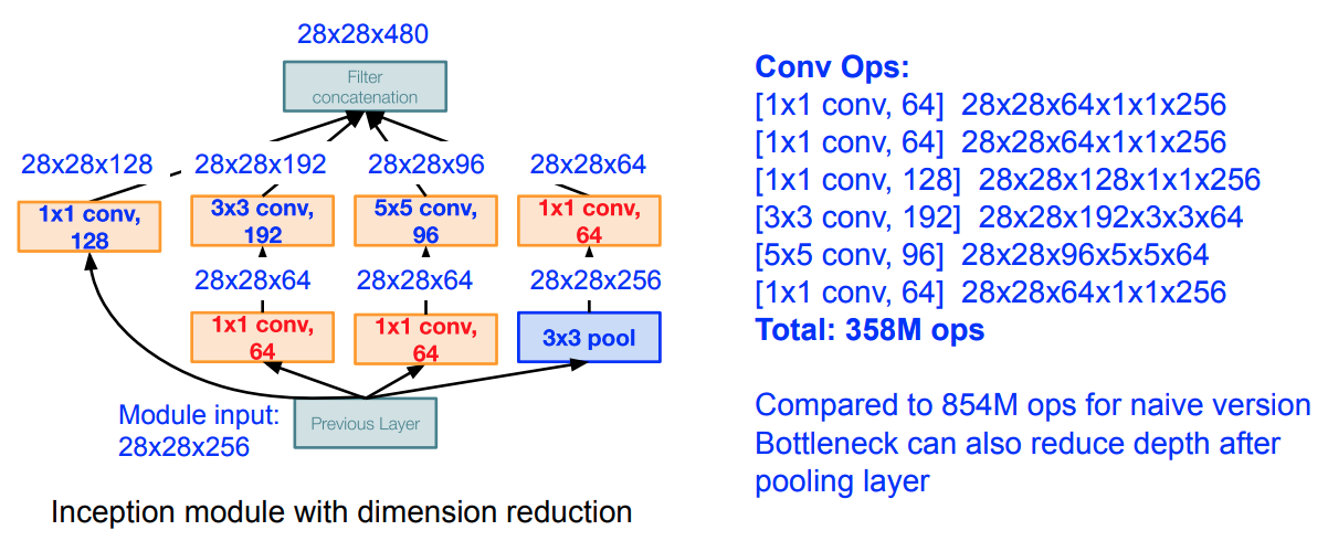
In this architecture, we have 12x less parameters than AlexNet.
ResNet
ResNet is yet another CNN architecture that drastically improve the error rate and won the ILSVRC-2015 with error of \(3.57\)%. It is a hugely deeper neural nets with 152 layers and uses residual connections.
So now you might be wondering, since deeper layers has demonstrated explicit improvement(as shown in VGGNet and GoogleNet), can we just make the neural net as deep as possible and achieve the best possible outcome?
The answer is NO.
The first obvious reason is overfitting right?
With the increase of parameters, the model starts to overfit in testing data. However, what’s strange about about it is that the training error for deeper layer is still higher.

So the hypothesis is that it is not caused by overfitting. Rather, it is an optimization problem, i.e harder to optimize.
An intuition is that the deeper model should be able to perform at least as well as the shallower model. Hence, a solution by construction is copying the learned layers from the shallower model and setting additional layers to identity mapping. ResNet uses the so-called residual block
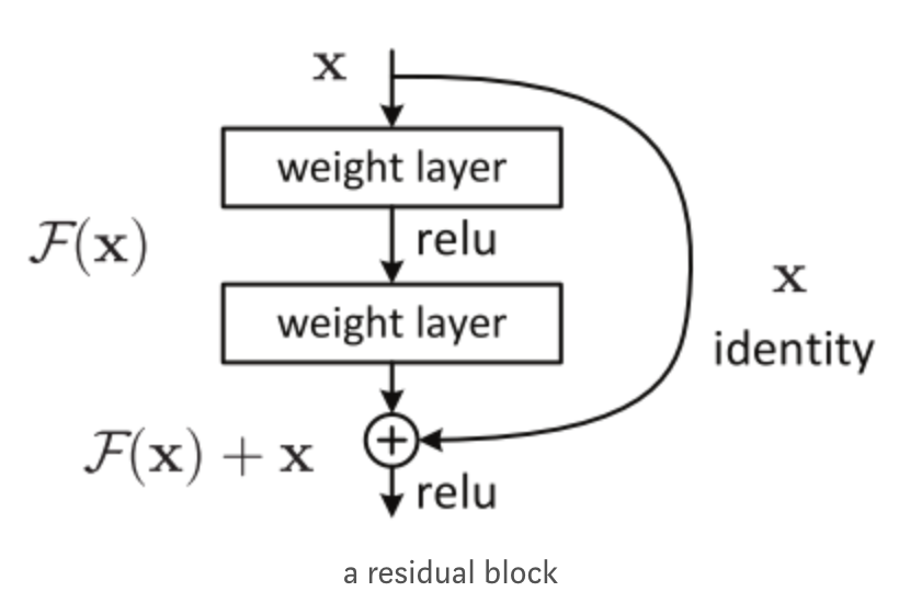
Instead of directly trying to fit a desired underlying mapping, use network layers to fit a residual mapping.
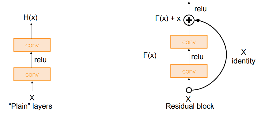
So the full ResNet architecture is
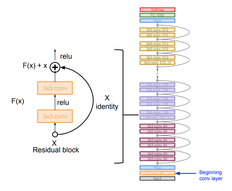
- Stack residual blocks
- Every residual block has \(2\) \(3\)x\(3\) conv. layers
- Periodically, double # of filters anddownsample spatially using stride \(2\)(/\(2\) in each dimension)
Here is the summary of ILSVRC and performance of different CNN architectures
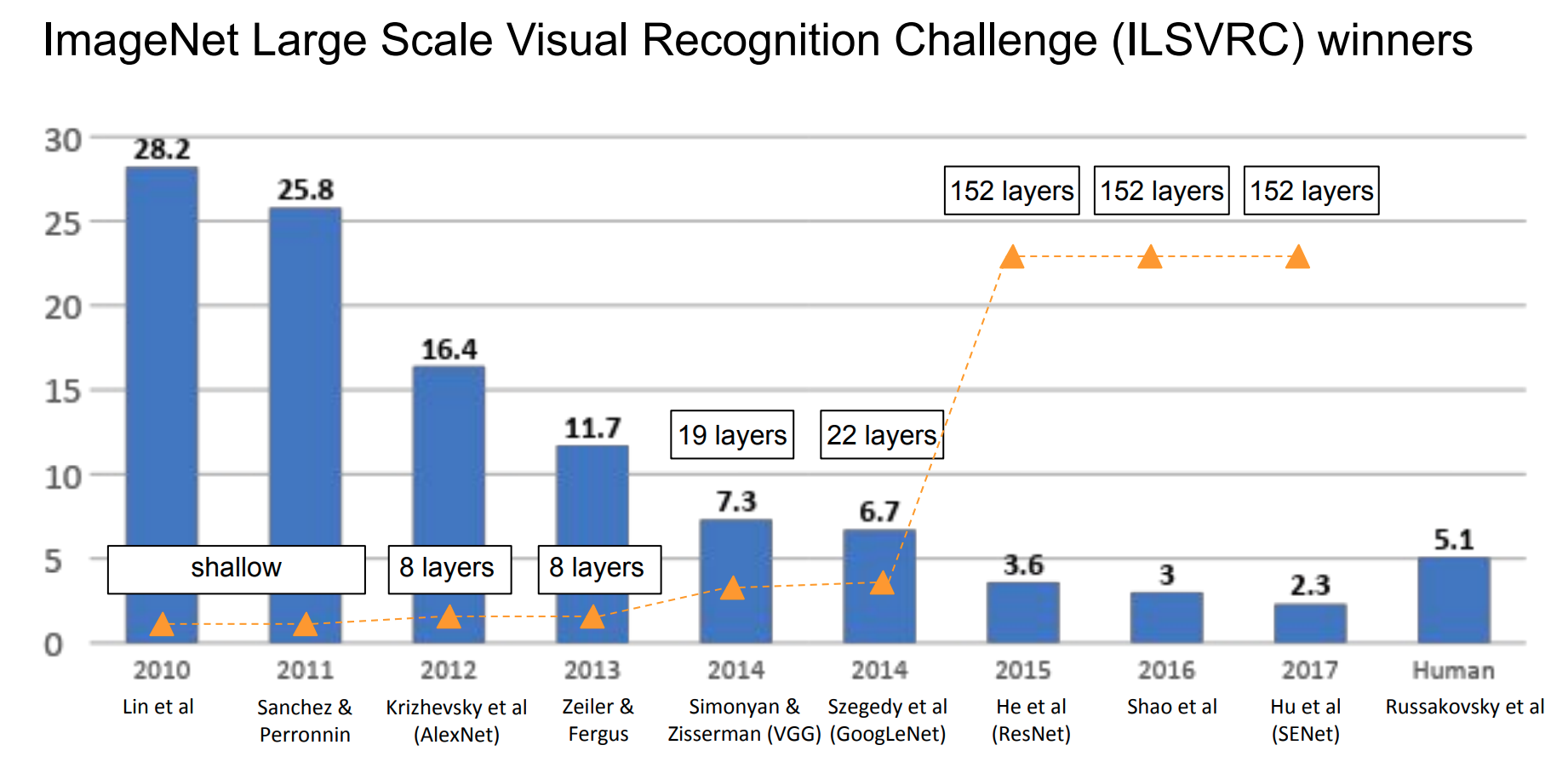
Ackownledge:Some AlexNet pictures and contents are adapted from SATYA MALLICK and some GoogleNet pictures are from Stanford CS\(231\)n.